Transformers

Modern Sequence Analysis

Nicholas Gale and Stephen Eglen

Traditional Sequence Analysis

• Sequence analysis has been typically performed by recurrent neural networks.

• Exploding/vanishing gradients from recursion.

• Information decay leading to short memory.

• O(n) complexity in sequence length.

Some solutions.

• LSTMs: forget gates to preserve information.

• Gated Recurrent Units: similar to LSTM forget gates but no output.

• Other proposals: none ideal due to O(n) complexity.

Transformers

• “Attention is all you need” (2016)

• Transformers are the latest development in large scale sequence analysis.

• Address many problems with RNNs

• Workhorse behind many “magical” applications e.g. voice assistant and language translation.

Attention: bare bones

• Transformers leverage the idea of attention: not new.

• Attention is computed between all elements in a sequence: a weighted relationship between locations.

• All units are considered independently: massive parallelisation.

Attention

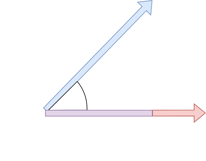
• Simple attention relies on nothing more than a Euclidean projection: dot product.

Simple attention: computation

• For each vector pair compute the dot product between them and normalise over all pairs with softmax. \[ a_{ij} = x_i^T x_j \] \[ A_{ij} = \frac{\exp(a_{ij})}{\sum_j \exp(a)_{ij}} \]

Attention Retrevial

• An input is weighted by the row of the attention matrix corresponding to its index.

• The ouput is the weighted sum of all vectors by this attention row: \[ y_i = \sum_j A_{ij} x_j \]

Querys, Keys, and Values

• Imagine the vectors are one-hot batched: \[(0,0,1, \ldots, 0,0)\]

• The product \(x_i^Tx_j\) will be one only in the indexes \(i=j\). Multiplying by the potential valus gives \(x_i\).

• This operation is acting like a look-up table.

• Transformers inherit the language and call these keys, queries, and values.

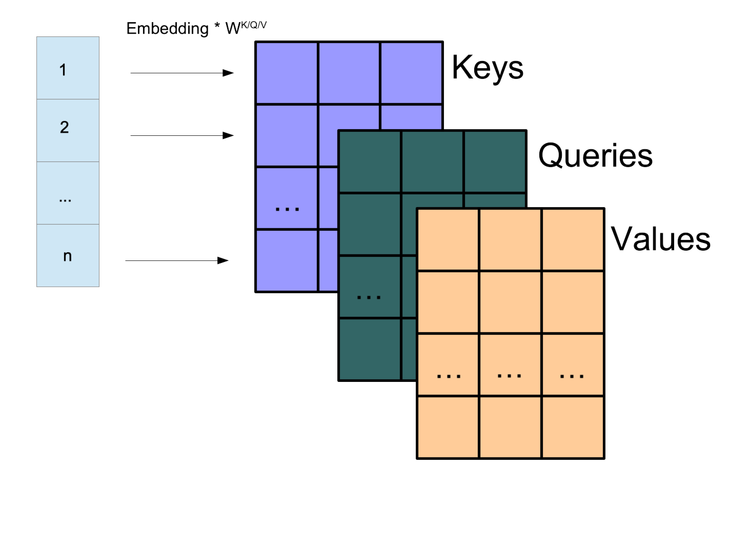
Attention Generalised

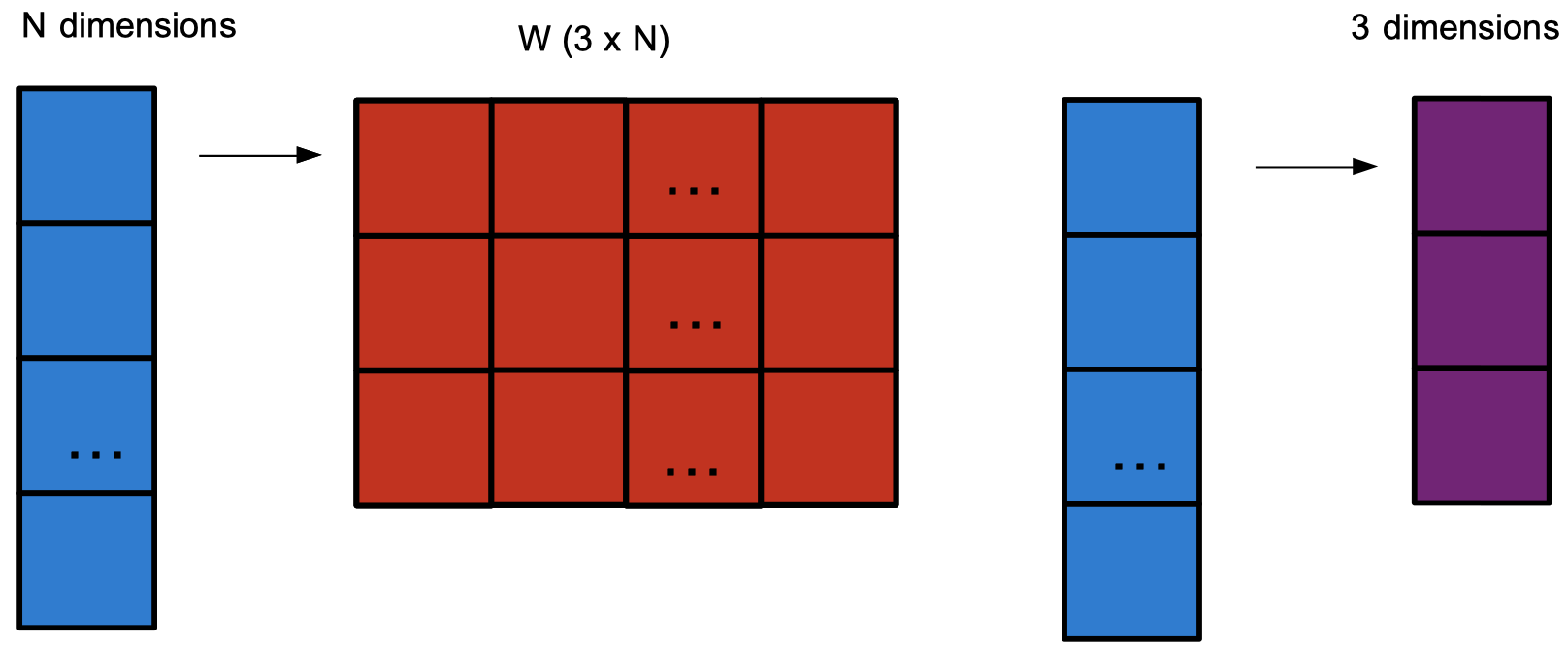
• We would like to let the keys, queries, and values not be fully determined by Euclidean representation.

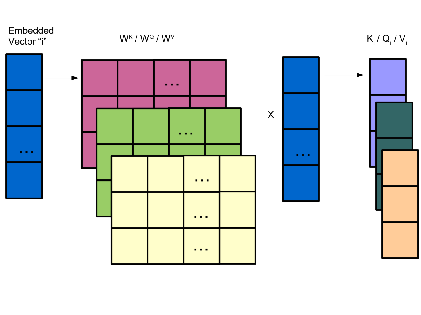
• We imagine them as linear transforms of the total dictionary embedding values into a new space: \[k_i = W^Kx_i, q_i = W^Qx_i, v_i = W^Vx_i\]

• This allows us to compress our key/query/value representation to a lower dimensionality.

Transformers Bare Bones

• The transformer model is composed of two attentional models: an encoder and decoder.

• Input is in the form of vectors of tokens e.g. genome sequence.

• The encoder transforms input to an encoded attentional sequence.

• The decoder autoregressively uses the encoder ouput to an ouput sequence.

• The output sequence is decoded with a decoder dictionary e.g. amino acids.

Transformers.jl

• Transformers.jl is built on top of Flux.

• It has similar GPU support (and similiar drawbacks).

• Similar grammar but there are subtleties - documentation is helpful!

• Open source contribution - documentation could be added to! Anyone can do this.

Transfomer Codon Task

• A codon is a group of three base nucleotides that encodes an amino acid.

• Can we try and predict amino acid base pairs without knowledge of codons?

using CSV, DataFrames, Transformers, Flux, Random, ProgressMeter

amino_codon = Dict( # the amino acid to codon relationship
    "A" => ["GCU", "GCC", "GCA", "GCG"],
    "R" => ["CGU", "CGC", "CGA", "CGG", "AGA", "AGG"],
    "N" => ["AAU", "AAC"],
    "D" => ["GAU", "GAC"],
    "B" => ["AAU", "AAC", "GAU", "GAC"],
    "Q" => ["CAA", "CAG"],
    "E" => ["GAA", "GAG"],
    "Z" => ["CAA", "CAG", "GAA", "GAG"],
    "G" => ["GGU", "GGC", "GGA", "GGG"],
    "H" => ["CAU", "CAC"],
    "I" => ["AUU", "AUC", "AUA"],
    "L" => ["CUU", "CUC", "CUA", "CUG", "UUA", "UUG"],
    "K" => ["AAA", "AAG"],
    "M" => ["AUG"],
    "F" => ["UUU", "UUC"],
    "P" => ["CCU", "CCC", "CCA", "CCG"],
    "S" => ["UCU", "UCC", "UCA", "UCG", "AGU", "AGC"],
    "T" => ["ACU", "ACC", "ACA", "ACG"],
    "W" => ["UGG"],
    "Y" => ["UAU", "UAC"],
    "V" => ["GUU", "GUC", "GUA", "GUG"],
    #"1" => ["AUG"],
    #"9" => ["UAA", "UGA", "UAG"],
);

Pre-Processing

• Token labels, a start/end symbol, and an unknown symbol are encoded into a lookup table (Vocabulary).

• The input sequence tokens are first wrapped by “Start” and “End” tokens and encoded by the Vocabulary.

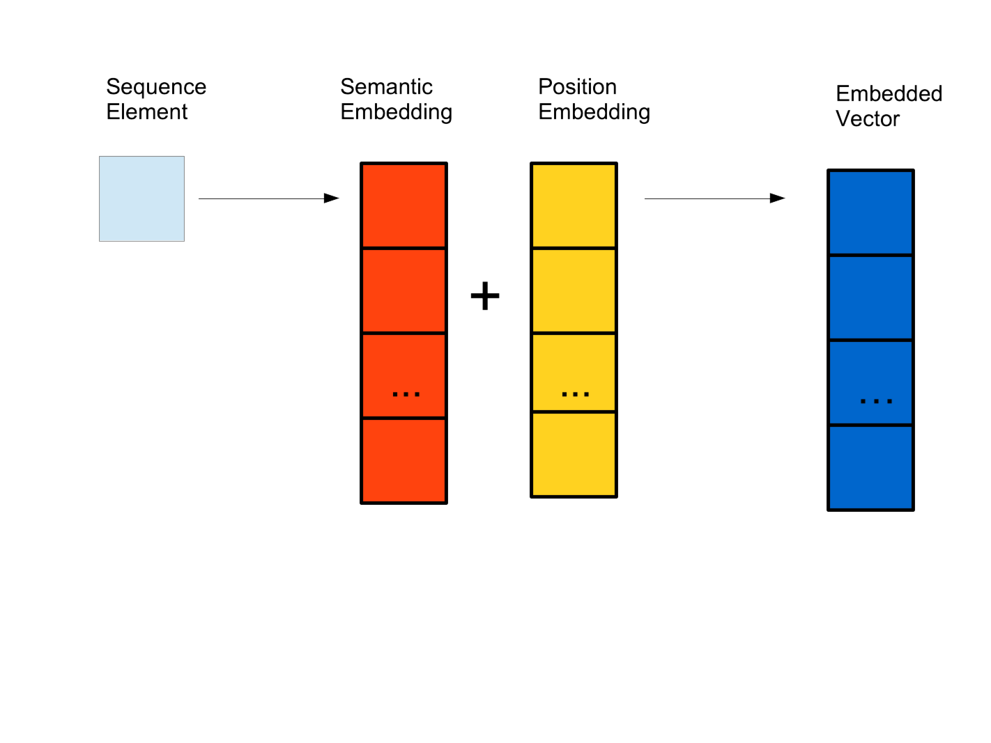
• This encoded representation is semantically embedded into vectors of length \(D\).

pre_process(v) = cat("1", v..., "9"; dims=1)
labels_y = cat("1", unique(train_y[1])..., "9", "0"; dims=1)
labels_x = cat("1", unique(train_x[1])..., "9", "0"; dims=1)
tokenizer_x = Transformers.Vocabulary(labels_x, "0")
tokenizer_y = Transformers.Vocabulary(labels_y, "0")
encoded_x = tokenizer_x.(pre_process.(train_x))
encoded_y = tokenizer_y.(pre_process.(train_y))
embed_x = Transformers.Embed(d, length(tokenizer_x))
embed_y = Transformers.Embed(d, length(tokenizer_y))

Positional Encoding

• Attention lets us forget sequence order to parallelise computation.

• Sequence orders are important e.g. gene sequence cant be scrambled.

• A positional encoding function is used to inject this order into the learning.

• Positional encodings can be learnt but typically use a function: \[ p_{2k}(i) = cos(i/10000^k) \] \[ p_{2k+1}(i) = sin(i/10000^k) \]

position_embed = Transformers.PositionEmbedding(d)

function embeddingx(x)
  sem_em = embed_x(x, inv(sqrt(d)))
  em = sem_em .+ position_embed(sem_em)
  return em
end

Keys, Queries, and Values

• The keys, queries and values are remembeddings of the information into a different representational subspace.

• These are the key learnable parameters in the model.

• An efficient subspace representation of information allows for impressive generalisability.

Attention Matrices

• Each input vector forms a row and these can be concatenated for efficiency into a matrix: \(X\) (L x D)

• K represents the keys, Q the querys, V the values.

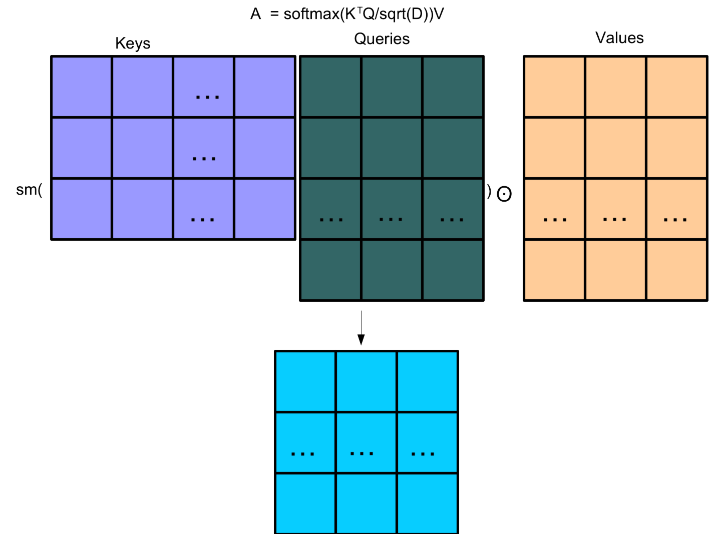
Transformer Attention Head

• The Transformer attention mechanism is given by: \[A(K,Q,V) = \text{softmax}\left(\frac{K^TQ}{\sqrt{D}}\right) \odot V\] \[K = W^KX, Q = W^QX, V = W^VX\]

• Softmax is calculated row by row. \(\odot\) is element-wise product. Dimensional scaling \(\sqrt(D)\) for stability.

Multi-head attention

• A transformer layer can have multiple heads analag. convolutional filter.

• Each of these heads will learn to focus on different semantic relationships.

• This can be efficiently encoded by simply concatenating each individual head. Usually, \(n \times h_d = D\).

• Head dimension is not a hyper-parameter.

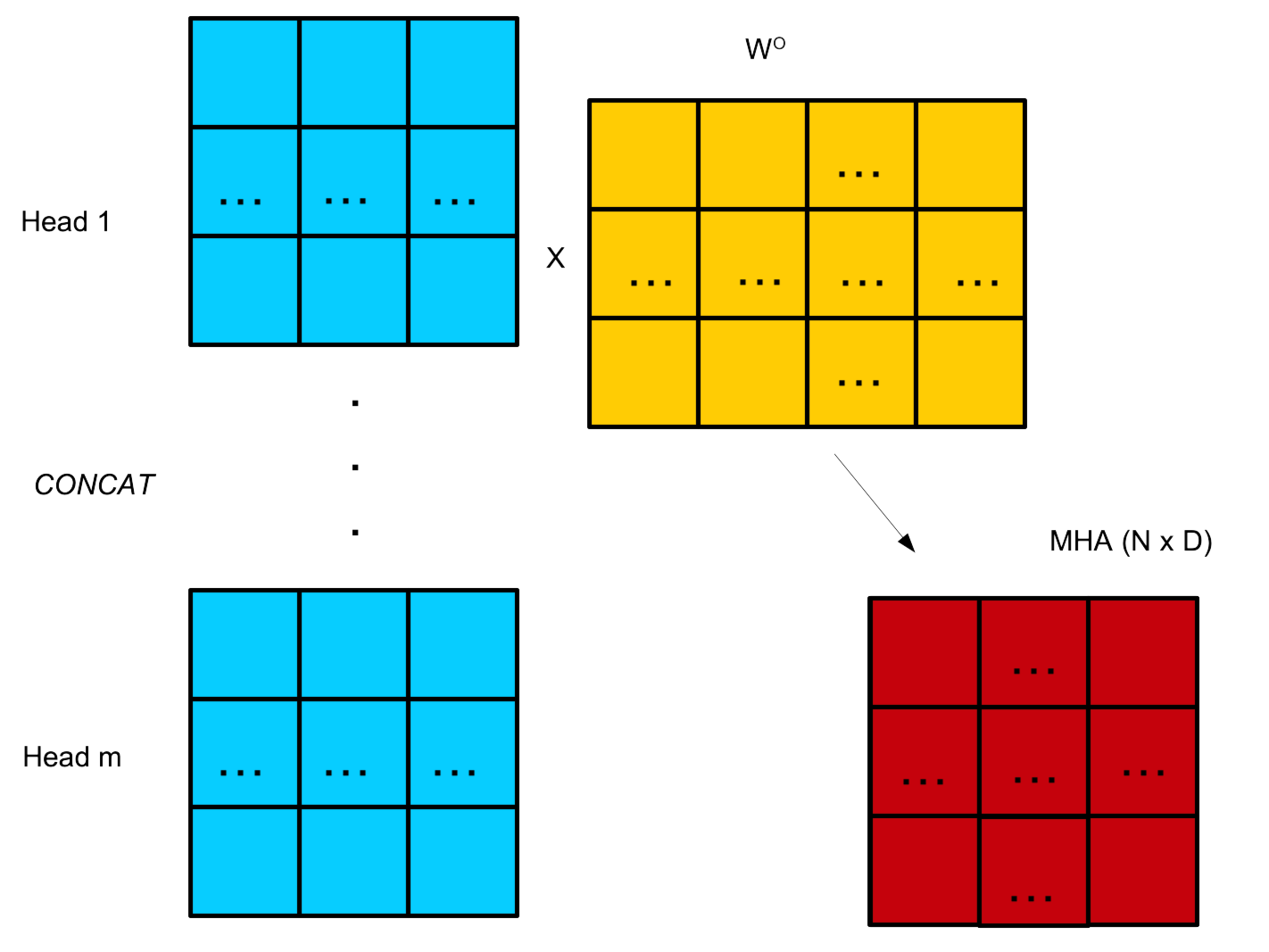
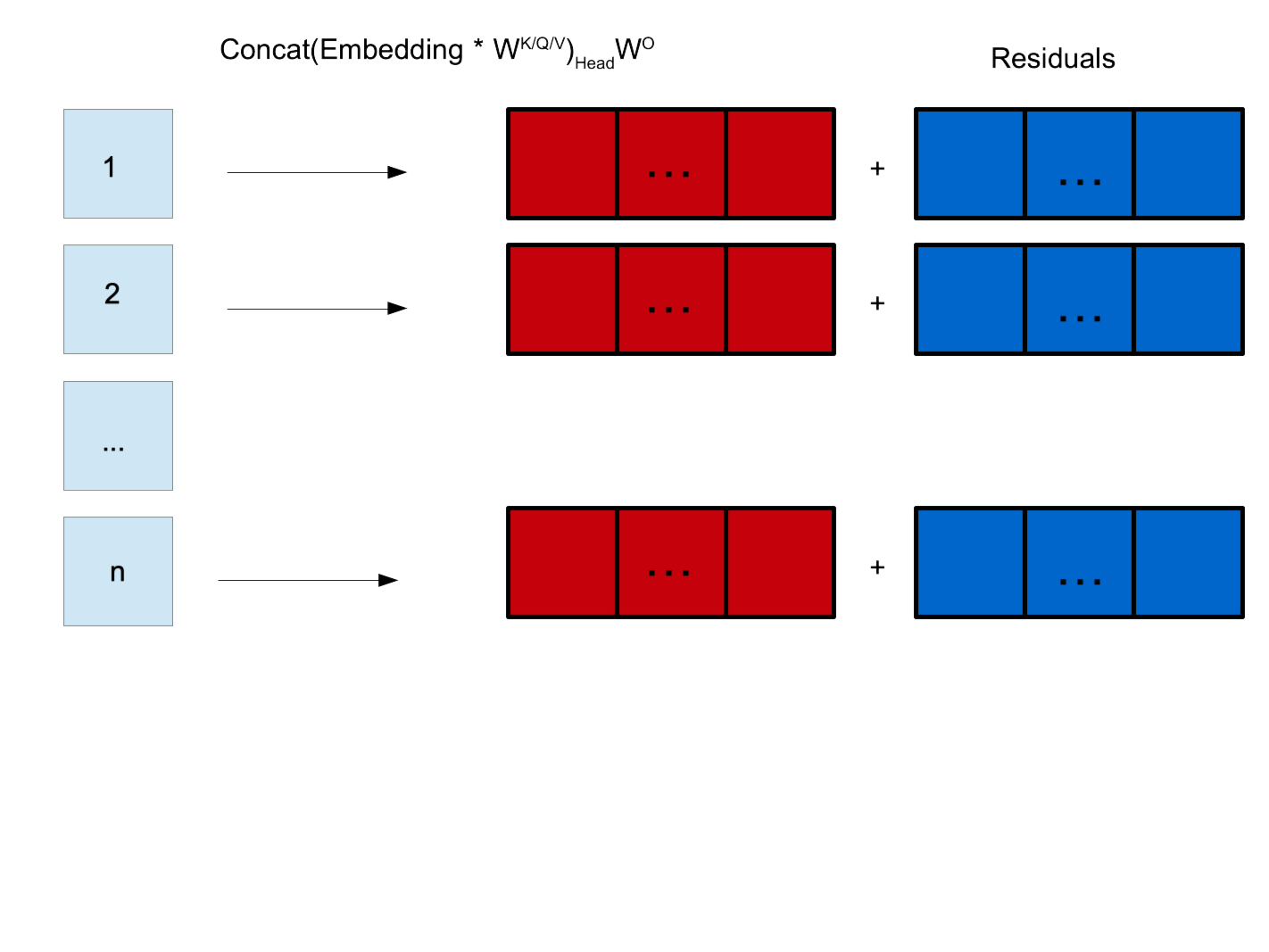
Residual and Normalisation

• The outputs of the attention mechanism are mutliplied by matrix \(W^O\) to remebbed vectors into length D.

• \(W^O\) is another learnable matrix.

• The pre-attention inputs (residuals) are added to the re-embedded attention transformed inputs.

• This combined vector is then layer-normalised.

Feed Forward Network

• The normalised self-attention and residuals are passed through a feed-foward network: \[F(x) = \text{ReLu}(W_1x + b_1)W_2 + b_2\]

Inner Dimensions

• The inner-dimension is independent of the embedding dimension e.g. 2048.

• The feed forward network is shared between all tokens.

• The residuals are added to the ouput of the FFN and layer-normalised.

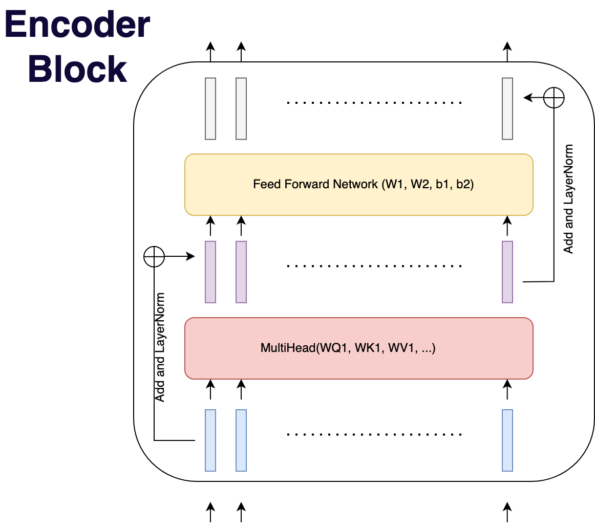
Encoder Block/Layer

• The operations of self-attention, feed forward networks, and layer-normalisation make an encoder block.

• This can be thought of as a layer in a regular NN.

• The Encoder is formed of several encoder blocks e.g. 6

Tencoder = Flux.Chain(
    embeddingx, 
    Transformer(d, h, hd, innerd), 
    Transformer(d, h, hd, innerd), 
    Transformer(d, h, hd, innerd)
)

Decoder Block

• A decoder block has a self-attention, an encoder-decoder-attention, and a feed-forward network.

• The encoder-decoder-attention keys and values are constructed using output from encoder (and learnable matrices).

• These keys and values are shared across all decoder blocks.

Dec1 = TransformerDecoder(d, h, hd, innerd)
Dec2 = TransformerDecoder(d, h, hd, innerd)
Dec3 = TransformerDecoder(d, h, hd, innerd)
ffn = Transformers.Positionwise(Dense(d, length(tokenizer_y)), softmax)

function Tdecoder((y, mx))
    emy = embeddingy(y)
    d1 = Dec1(emy, mx)
    d2 = Dec1(d1, mx)
    d3 = Dec1(d2, mx)
    ffn(d3)
end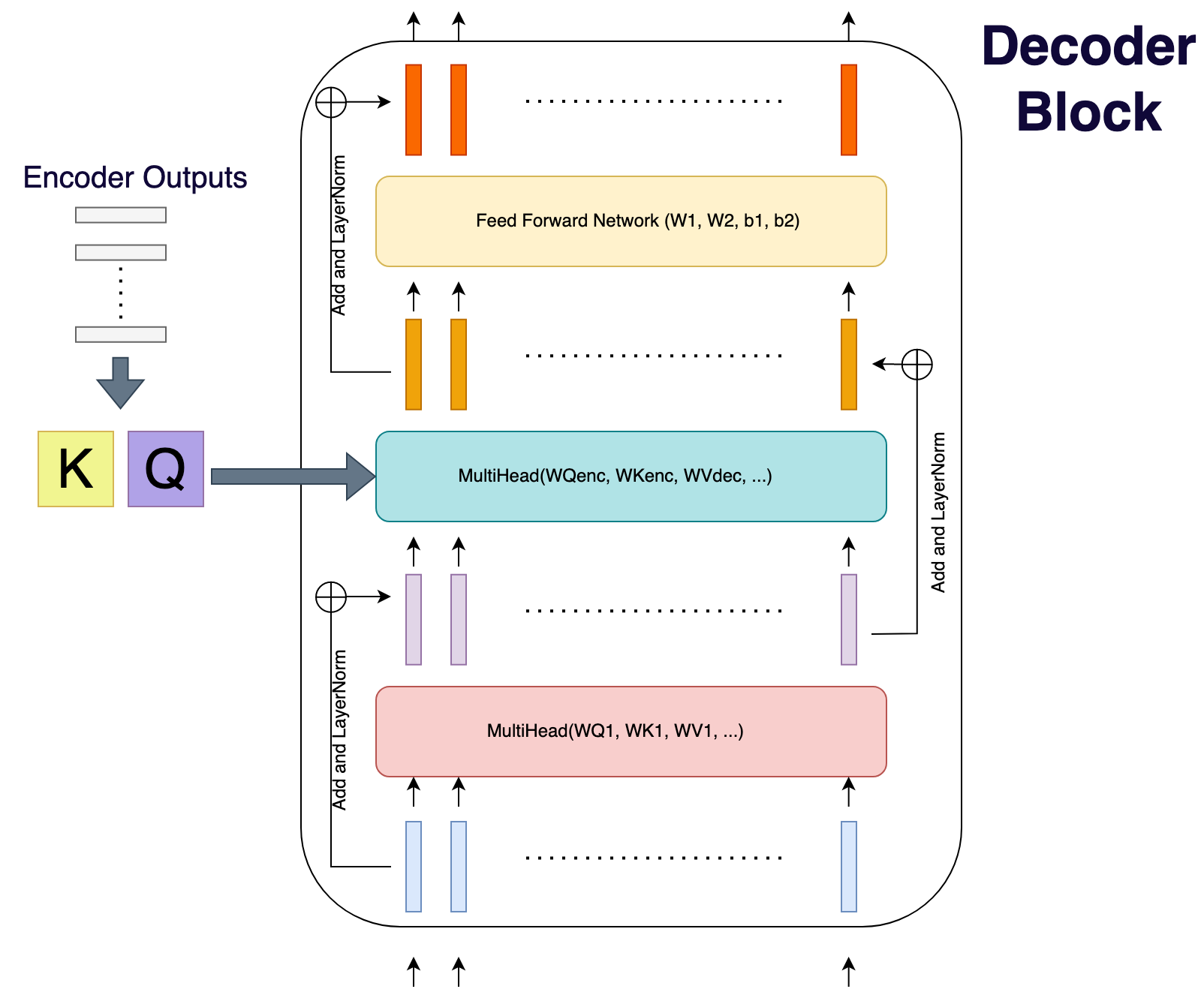

Sequence Generation

• Sequences are generated with a start symbol and terminated with a stop symbol.

• The outputs are fed through the network as inputs until stopping.

• The output vector is fixed at an arbitrary length i.e. 1024

• Future outputs are masked with -Inf to prevent left flowing information: autoregressive.

function transcribe_protein(x)
    seq = [tokenizer_y("1")]
    tok = ["1"]
    enc = Tencoder(x)
    for i = 1:2*length(x)
        dec = Tdecoder((seq, enc))
        seqnext = argmax(vec(dec[1:end-1,end]))
        append!(seq, seqnext)
        toknext = Transformers.decode(tokenizer_y, seqnext)
        push!(tok, toknext)
        toknext == "9" && break
    end
    tok
end

Loss Functions

• The final step is to softmax outputs to generate a probability distribution against a dictionary/vocabulary.

• The natural loss function is crossentropy.

• Loss functions may be arbitrary.

Regularisation

• The original paper used dropout for the layer parameters and label smoothing.

• Dropout improves stability and convergence time.

• Label smoothing increases model perplexity (at the cost of labelled accuracy).

function loss(xdata, ydata)
    L = 0
    for i in 1:length(ydata)
        ytarget = Flux.label_smoothing(Flux.onehot(tokenizer_y, ydata[i]), 0.2f0)
        ypred = Tdecoder((ydata[i], Tencoder(xdata[i])))
        L += Flux.crossentropy(ytarget, ypred)
    end
    return L
end

Model Summary

• The encoder takes positional and contextual inputs and the decoder autoregressively produces outputs.

• The encoder and decoders use attention heads and a feed-forward network to perform the learning.

• The attention mechanism transforms embedding into a different subspace through keys/queries/values matrices.

• Keys, Queries, Values are learned and represent optimal information relationships in the problem context.

Transfer Learning

• Transformer models are large - amongst the largest neural networks.

• Difficult to train without industrial resources.

• Employ transfer learning: import pre-trained weights on a similar task and fine-tune to current task.

Transformers in Biology

• Transformers are in relative infancy - lots of work to be done.

• The obvious candidate is sequence analysis: genome and protein.

• Some interesting developments: gene transcription factors using Enformer (Deep Mind)

• Protein Prediction tasks.

Transforming the Language Of Life.

• Protein prediction can be done classically: HMMs and BLAST. Exponentially computationally expensive.

• CNNs and RNNs are computationally more efficient but task depedent and dont generalise.

• Authors propose Transformer model PRoBERTa: pre-trained agnostic amino acid sequence representation.

• Protein prediction tasks: binary PPI and protein family classification.

PPI = prediction of protein interactions

Problems

• Authors managed to achieve state of the art performance on target tasks (tasks not too important)

• The resulting model is vastly more computationally efficient: 128 GPUs for 4 days => 4 GPUs for 18 hours.

• Still difficult to reproduce. GPUs are top of the line and few people have access to this many.

• Transformers in general are large models and pose a reproducibility problem.

Summary

• Transformers are a complex but powerful sequence analysis architecture.

• Julia offers support through Transformers.jl.

• Very successful, but computationally demanding and not easily reproducible.

• Relatively unplumbed in Biology.

References

Attention is all you need; Vaswani et. al. (2017)

Effective gene expression prediction from sequence by integrating long-range interactions; Avsec et. al. (2021)

Transforming the Language of Life: Transformer Neural Networks for Protein Prediction Tasks; Nambiar et. al. (2020)