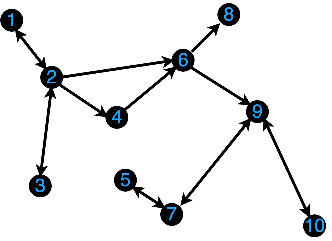
10×10 Matrix{Int64}:
 0  1  0  0  0  0  0  0  0  0
 1  0  1  1  0  1  0  0  0  0
 0  1  0  0  0  0  0  0  0  0
 0  0  0  0  0  1  0  0  0  0
 0  0  0  0  0  0  1  0  0  0
 0  0  0  0  0  0  0  1  1  0
 0  0  0  0  1  0  0  0  0  0
 0  0  0  0  0  0  0  0  0  0
 0  0  0  0  0  0  1  0  0  1
0 0 0 0 0 0 0 0 1 0Graph Neural Networks
The Blueprint Neural Networks
Graphs
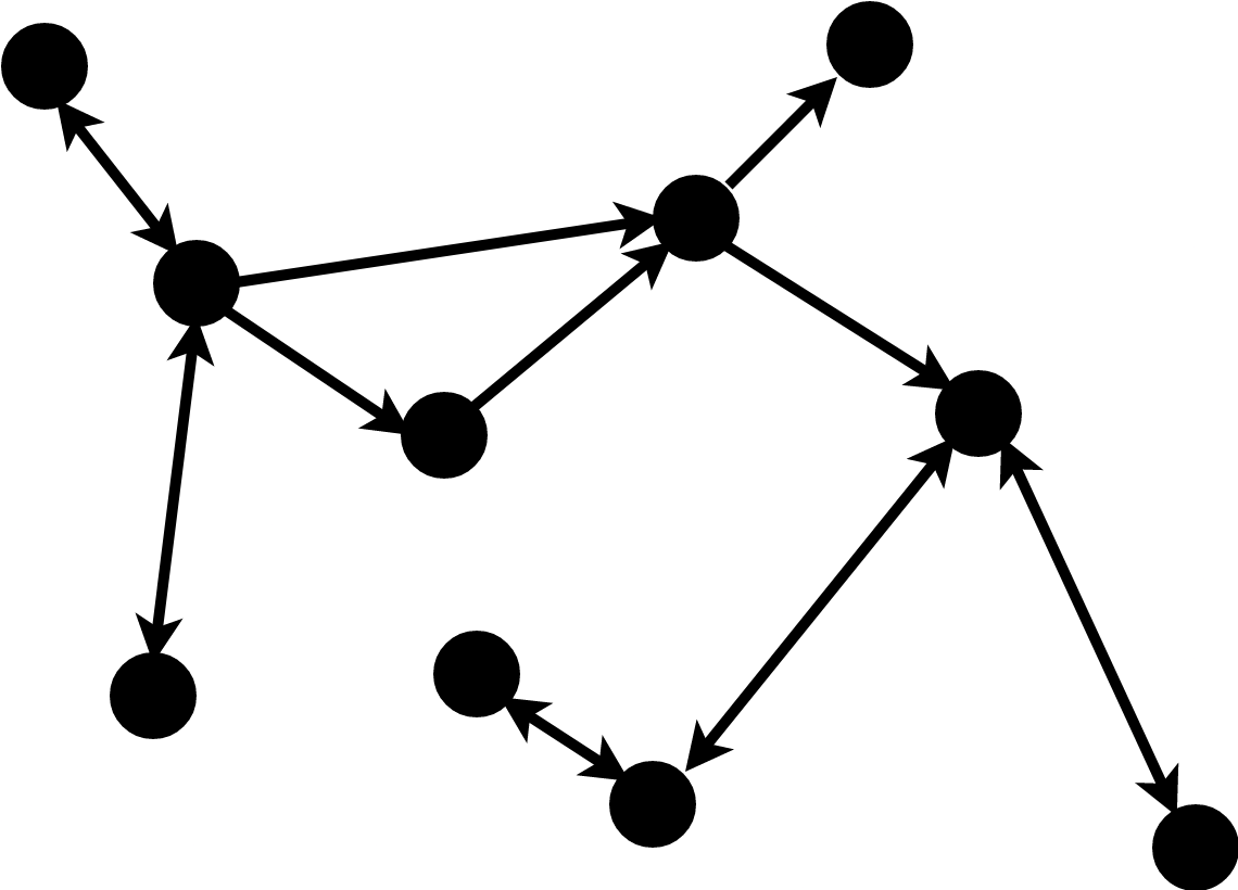
Graphs in Science
Naturally intuitive way to represent objects e.g. molecules.
Graphs are generalised non-linear data structures e.g. gene regulatory networks.

Formal Definitions
A graph \(G\) is an tuple of nodes \(V\) and edges \(E\): \((V,E)\).
The nodes are labelled \(\{1, 2, \ldots, N\}\).
The edges are weighted relationships between nodes: \(1 \mapsto 4\) etc.
Adjacency Matrix
An adjacency matrix an object capturing node-edge relationships.
The rows/columns are the vertex index.
The matrix value \(w_{ij}\) is the edge weight between \(i\) and \(j\).
Feature Matrix
Graphs can be equipped with a feature matrix to hold data.
Each node encodes a vector of \(F\) measurable features: weight, chromosome number, membrane voltage, etc.
The feature matrix is the \(N \times F\) matrix of concatenated features.
Neighbourhood
The neighbourhood of a node \(i\) is denoted \(\mathcal{N}(i)\).
The in neighbourhood is all the nodes with edges flowing into \(i\).
The out neighbourhood is all the nodes with edges from \(i\). \[\mathcal{N}(i) = \{ j : (ij) \in E \}\]
Permutation Invariance
A permutation is a relabelling of a graph nodes.
A permutation matrix \(P\) reshuffles an adjacency matrix: \(P^{-1} A P\).
Reshuffle feature data by \(P^{-1} F_M\).
Changing graph labels doesn’t change graphs.
Analysis functions should also be permutation invariant e.g.
sum
Neural Networks
We now want to define a neural network on these graphs.
Our input is the graph and the feature matrix of data.
We transform inputs \(x_i\) on the nodes to latents \(h_i\) through a neighbourhood invariant function \(g\)
Julia Graph Neural Networks
GraphNeuralNetworks.jlpackage is built on top of Flux.Excellent support for many layer types and documentation.
Models are composed with
GraphNeuralNetworks.GNNChain.
Specifiying Graphs
Graphs are specified with
GNNGraph(obj)Objects can be adjacency matrices, adjanceny lists, and COO representation.
Feature data (last dim = nodes) is passed with the
ndatakeyword which can be an optionally named tuple.
using GraphNeuralNetworks, Flux
amat = [
    0 0 1 0;
    0 0 1 1;
    1 1 0 0;
    0 1 0 0
    ]
alist = [[3], [3, 4], [1, 2], [2]];
coo_source, coo_target = [[1, 2, 2, 3, 3, 4], [3, 3, 4, 1, 2, 2]]
g1 = GNNGraph(amat); g2 = GNNGraph(alist); g3 = GNNGraph(coo_source, coo_target);
@show adjacency_matrix(g1) == adjacency_matrix(g2) == adjacency_matrix(g3)

GNNGraph(amat, ndata = rand(Float32, 10,4))
GNNGraph(amat, ndata = (; x=rand(Float32, 10, 4), pr=rand(Float32, 2, 4)))
adjacency_matrix(g1) == adjacency_matrix(g2) == adjacency_matrix(g3) = trueGNNGraph:
num_nodes = 4
num_edges = 6
ndata:
x => 10×4 Matrix{Float32}
pr => 2×4 Matrix{Float32}Pooling
Pooling is a graph reduction method.
It is implemented as a layer in a graph neural network.
Commonly, aggregrate features of subset of nodes to produce a new graph.
GlobalPoolaggregates to a single feature matrix.
Types of GNNs
There are many different types of GNNs. Historically, and currently.
They usually share many similarities but different names.
Generally three types: Convolutional, Attentional, and Message Passing.
Convolutional
Features are embedded into some latent space through a shared feature transformation \(W\).
We aggregate the sum of features of nodes neighbourhood (usually node inclusive) multiplied by some weighting factor \(\alpha_{ij}\) (usually \(1/\sqrt(|N_i||N_j|)\)).
It doesn’t need to be a sum (any permutation invariant function will do). \[h_i = f\left(\sum_{j | (i,j) \in E} \alpha_{ij} W x_j \right) \]
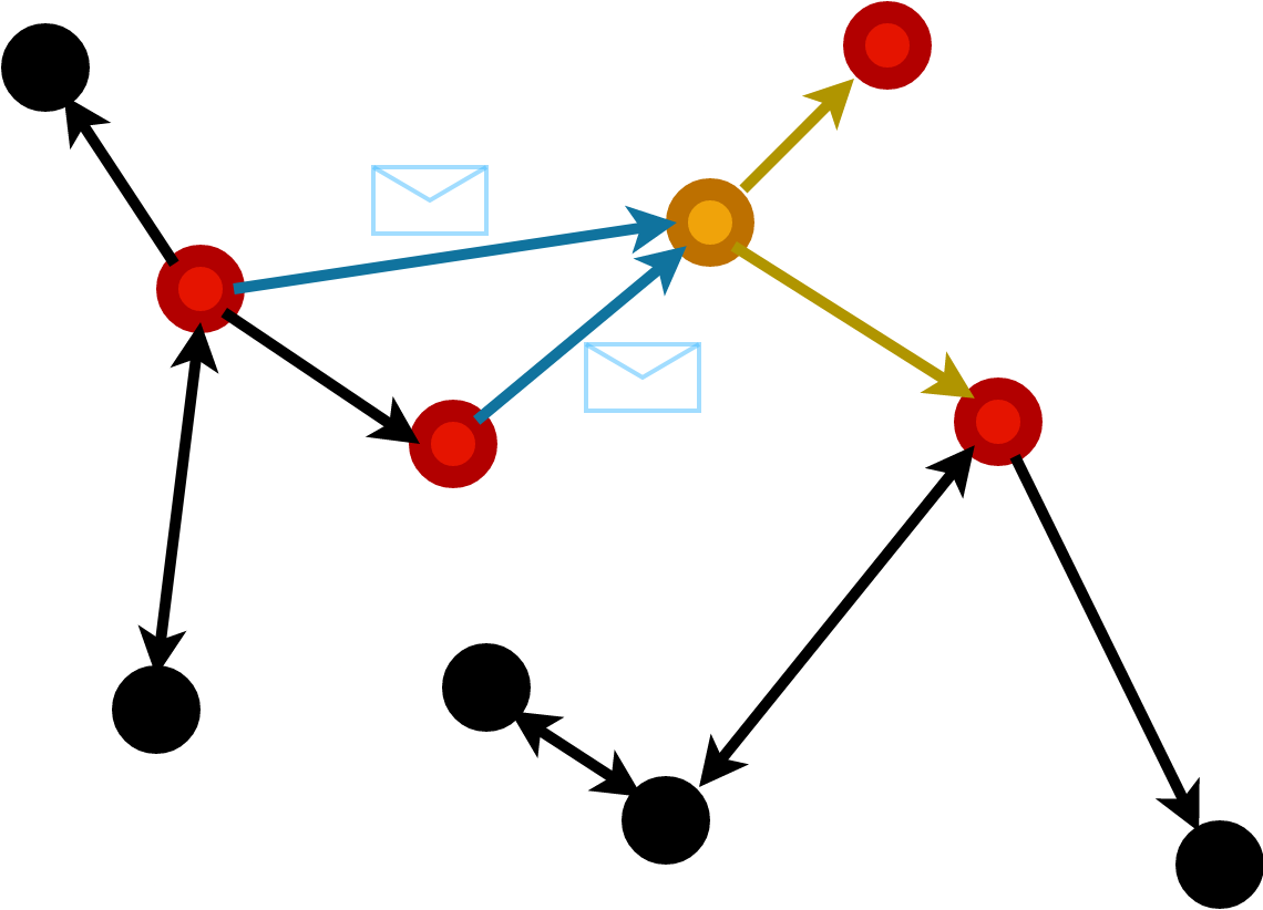
Convolutional GNNChain
Specified by latents in and latents out.
API call is
GCNConv(in => out).
Attentional
We perform a similar procedure but allow the normalising weights to be dynamic.
Attention is constructed over the feature weights of a nodes neighbourhood.
They are therefore functions dependent on data and learnable: \[ h_i = f\left(\sum_{j | (ij)\in E} \alpha(x_i, x_j) W x_j \right) \]
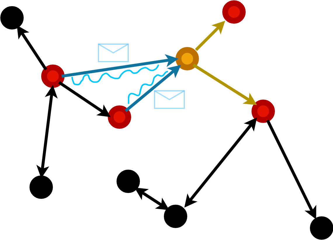
GATConv
The graph attention network is the most common in use today.
Specified by latents in (and edge features in) to latents out with keywords
σ,bias,heads,init,negative_slope,add_self_loops.
Message Passing
Compute message vector to be sent along an edge dependent on receiver and sender node features and edge features.
The messages from each node are aggregated to form the readout.
Most generic form of graph network \[ h_i = f\left(x_i, \sum_{j | (ij) \in E} \phi(x_i,x_j) \right) \]
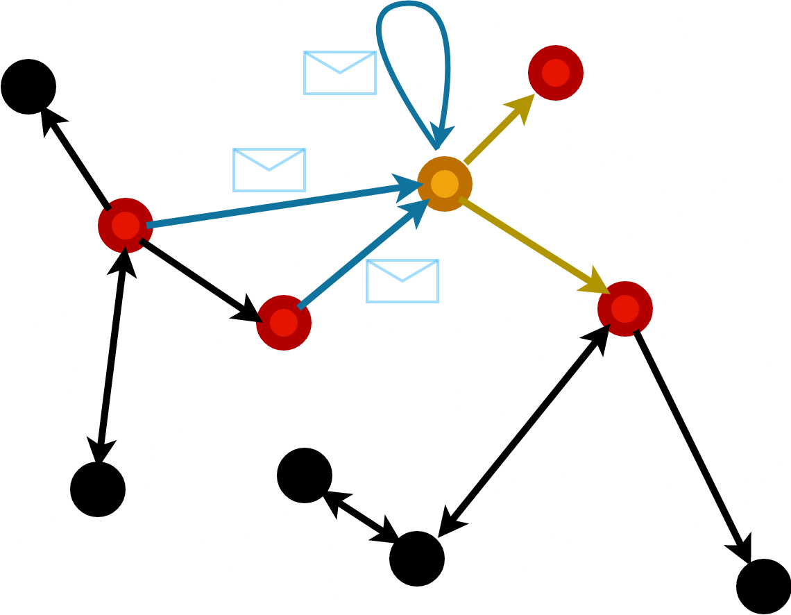
Message Passing
Define a message function on nodes and edges: \(f\).
Choose an aggegration function e.g.
sum,meanetc.Define a graph and choose graph layer.
Apply message to edges with
propagate(f, Graph, aggr)
State update and objective.
Early GNNs (1980s) applied update rule to latents until convergence.
Modern GNNs do it a fixed time e.g. 5 or 20.
Latent states are used to feed another layer, or train an objective: regression or classification.
Node classification / regression: \[p(h_i) \in \text{Category Set} / \mathbb{R}^n\]
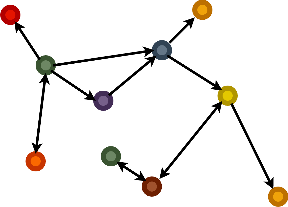
Graph classifcation / regression: \[p(G) \in \text{Category Set} / \mathbb{R}^n\]

Link Prediction: \[p(i,j) = e_{ij}\]
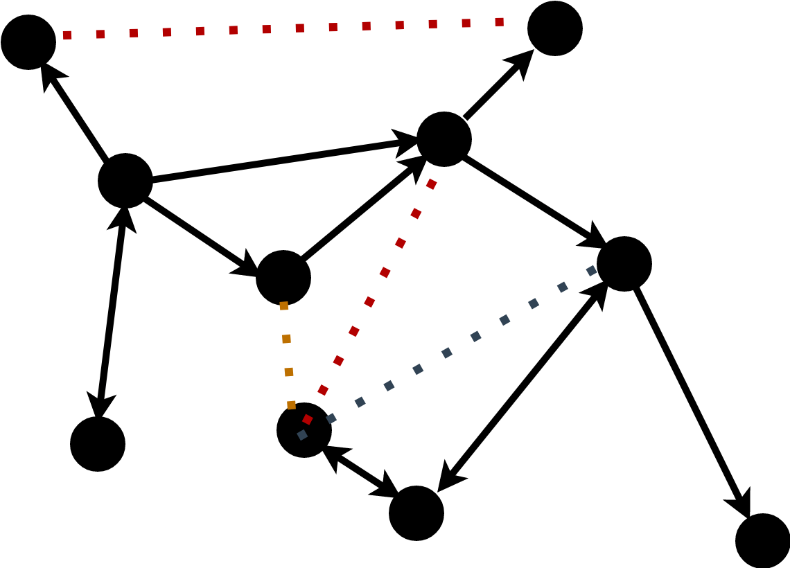
Loss Functions
These are normally trained on a classifier (dense) network on the latents.
The loss functions for GNNs must be permutation invariant.
Loss is chosen to be objective appropriate e.g. MSE.
Batching and Padding
A set of graphs might have variable numbers of nodes.
A solution is to appropriately pad adjanceny matrix with zeros.
A block matrix has matrices embedded in a matrix:
Wb = [W1 W2; W3 W4].A block diagonal matrix with
W2=W3=0will preserve the structure of W1 and W2.
Computationally
Batch all graphs into a single graph.
Use a data loader object to perform stochastic gradient descent.
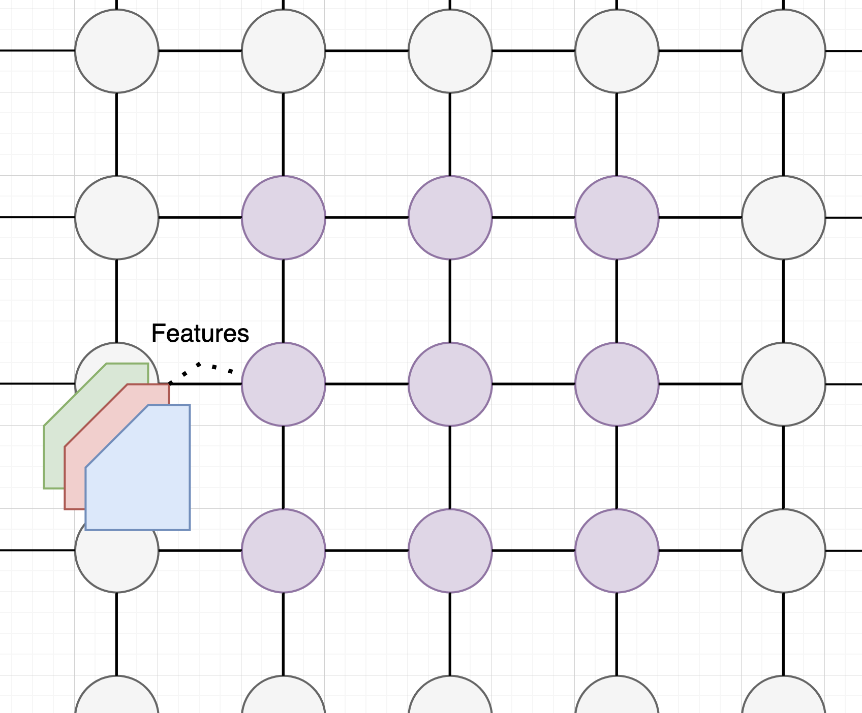
ConvNets: A familiar smell
We have already covered a form of GNNs: the conv net.
The data structure is a grid topology: the edges are bidirectional in neighbouring pixels.
The message passing happens through the convolutional filters.
Recurrent Nets: A familiar smell.
Another form of GNNs covered is the RNN.
Line graph: each node has two edges for the data before and after i.e. a sequence.
Message passing happens through the internal and input states.

Generalised Neural Networks
All of our current neural network topologies can be expressed as GNNs
Formally: all networks can be generated by considering the symmetries and actions of a graph.
It’s still often better to use optimised pipelines
An eye on the future
The generalisation of neural networks is a recent field: Geometric Deep Learning.
It has generated a lot of interest recently.
Looks poised to be well suited to biological data.
All neural networks are generated by considering underlying symetries of a graph e.g. Translational Invariance => CNN.
Package:
GeometricFlux.jl
Halicin: a Halo Example
Chemicals have a natural graph structure: represented by bonds.
Train on a known set of working drugs.
Regression on space of potential drug molecules to perform drug screening/discovery.
Summary
Graphs are generalised forms of natural data: molecules, brains etc.
Graphs are defined by their adjacency matrix.
GNNs are graphs with features defined from data.
A GNN computes several passes of a message through the graph. The latents perform some learning task.
References
A Deep Learning Approach to Antibiotic Discovery; Stokes et. al. (2020)
Geometric Deep Learning; Bronstein et. al. (2021)