Generative Adverserial Networks

Generative Modelling with Neural Networks

Nicholas Gale and Stephen Eglen

What are GANs

• GANs are a generative model of neural networks

• They learn a statistical distributions properties.

• They can then be used to generate samples from that distribution.

• Famous examples are style transfer and face generation.

The Basic Idea

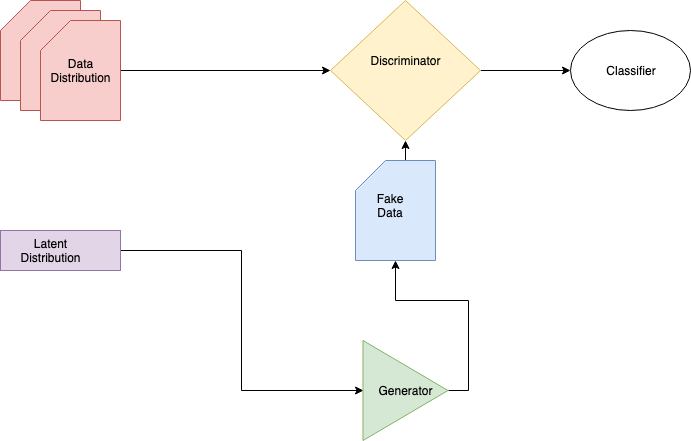
• A GAN is really a composition of two models: a generator and a discriminator.

• The generator is trained to trick the discriminator.

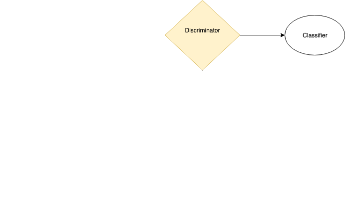
• The discriminator is trained to filter real data from fake.

• The goals are opposed: adverserial.

Components

• Suppose the data are generated from some distribution: \[ x \sim \text{Dist}(\alpha...) \]

• The discriminator is a function mapping to a binary target: \[ D \rightarrow \{ 0, 1 \} \]

• The generator \(G\) takes a latent vector \(z \sim U(0,1)^k\) and generates a fake data sample: \[G(z) = y \sim \text{Dist}_\text{Gen}(\alpha^\prime \ldots) \]

• The training goal is to approximate the data generating distribution: \[ \text{Dist}_\text{Gen}(\alpha ^\prime \ldots) \approx \text{Dist}_\text{Data}(\alpha \ldots) \]

• We are always interested in some data generating distribution.

• The discriminator needs to be trained to see if the data is real (1) or fake (0)

• The generator needs to trick the discriminator and is a probability distribution from a random variable \(Z \sim U(0,1)^k\).

• The latent space is commonly uniform between 0 and 1. More dimensions are added for complexity.

Construction

• \(G\) and \(D\) are arbitrary probability transforms.

• Neural networks are common choices: generalised functions.

• Desirable to use data to inform network architecture.

Loss Functions

• The discriminator is acting as a binary classifier.

• The natural loss function is logitcrossentropy: \[ L = -E_{x\in\text{Dist}_\text{Data}} [\log(D(x))] - E_{y \in \text{Dist}_\text{Gen}}[\log(1-D(G(z))]\]

Discriminator Loss

• The discriminator aims to minimise the above loss.

• The generator is targeting a vector in the data distribution.

• For labelled data \((x,y)\) this reduces to: \[ L_D(x, y) = -y\log(D(x)) - (1 - y) \log(1 - D(x))\]

Generator Loss

• The generator is aiming to trick the discriminator.

• Natural reward is to flip the classification loss.

• It doesn’t need to know the data: this is implicitly learned. \[ L_G(z) = -\log(D(G(z))) \]

• Implicit learning is good

• You cant just learn the copy function from available data

Training

• Training proceeds in a two-step fashion.

• First, batches are presented to the generator and G updated.

• Second, batches are presented to discriminator and D updated.

A simple example

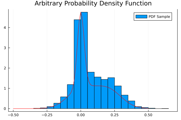
Consider a non-trivial probability distribution:

Training Code

D(samples) = Chain(Dense(samples=>100, relu), Dense(100=>50, relu), Dense(50=>1, σ))
G(input, samples) = Chain(Dense(input=>50, relu), Dense(50=>1000, relu), Dense(1000=>samples, x->0.5*tanh(x), bias=false))
lossD(x, y, dsc) = -mean(y.*log.(dsc(x))) .- mean((1 .- y).*log.(1 .- dsc(x)))
lossG(z, gen, dsc) = -.mean(log.(dsc(gen(z))))

# Training functions
function train_discriminator(dsc, gen, gendata, real_data, batch, opt)
    data = DataLoader(hcat(gendata, realdata), batchsize=batch, shuffle=true)
    Flux.train!(lossD, Flux.params(dsc), data, opt)
    Flux.train!(lossG, Flux.params(gen), gendata, opt)
end

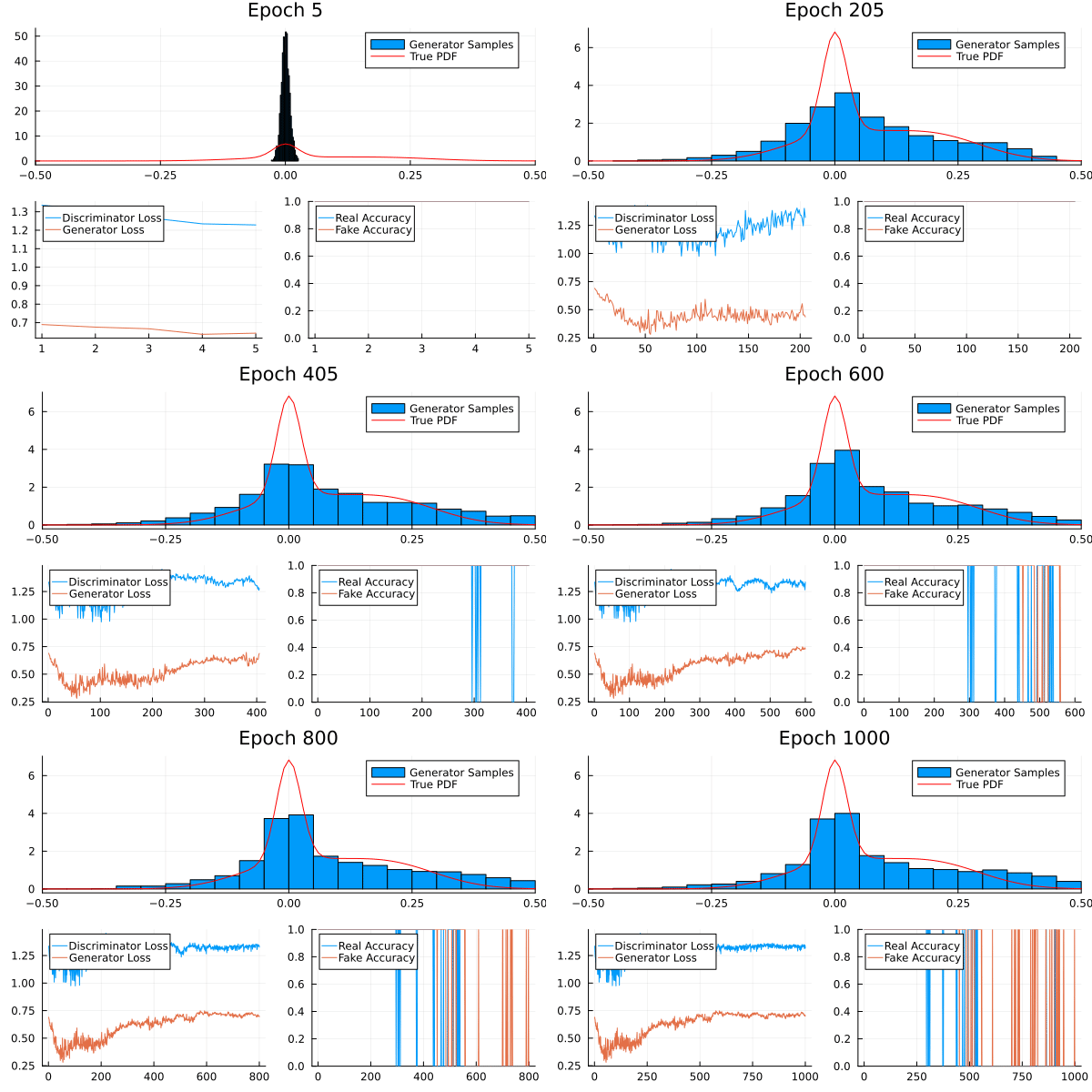
Result

Game Theory

• \(G\) and \(D\) are playing a two player game.

• This loss function is a min-max game.

• Training converges to a Nash equilibrium.

• The global minima of the game is \(\text{D}_\text{Data}(\alpha \ldots) = \text{D}_\text{Gen}(\alpha^\prime \ldots)\)

MNIST

• A famous dataset of handwritten numbers.

• Very common machine learning benchmark.

• MNIST Sample

Instability

• GANs are difficult to train even on simple data such as MNIST.

• Getting a GAN to converge is often a case of “machine teaching”.

• This is valuable in and of itself - helps construct the mental model of the problem.

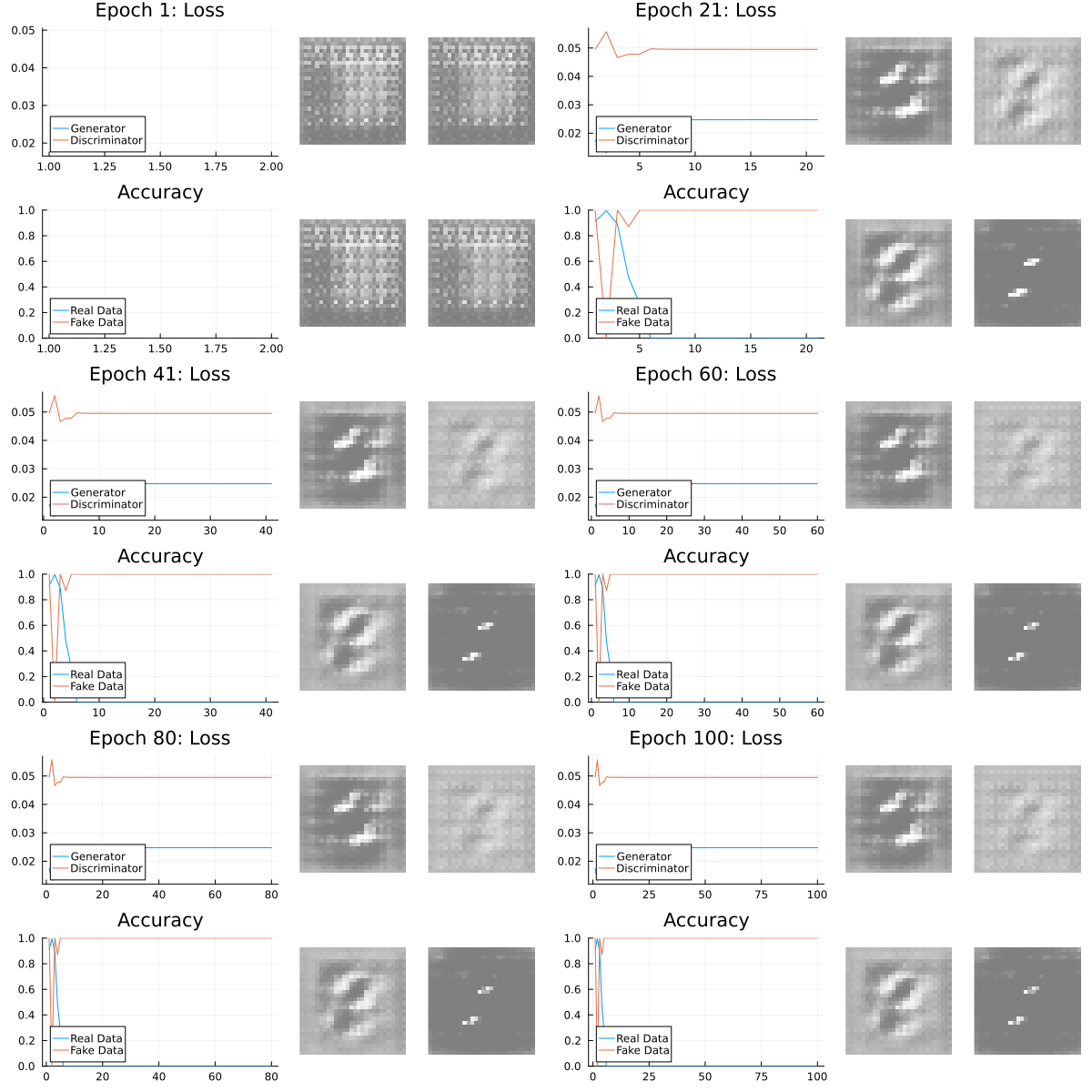
• There are some common GAN instabilities: saturation and mode collapse.

Loss Saturation

• The min-max loss function often saturates: the gradients go to zero.

• This can happen when the discriminator gives an overly confident rejection.

• Less of a problem with Wasserstein Loss GANS.

Loss Saturation

Saturation Fixes

• Adjust learning rate down for the discriminator.

• Change discriminator complexity.

• Apply dropout and other regularisation techniques.

Mode Collapse

• The generator doesn’t know the variability of the data.

• It can produce a very reliable subset which tricks the generator.

• This is known as mode-collapse: the target data is a composition of modes.

Mode Collapse

Mode Collapse Fixes

• Increase latent size: more degrees of freedom to optimise.

• Modify optimiser and learning schedule: a slower rate helps.

• Regularisation: dropout and normalisation are useful.

Training Practice

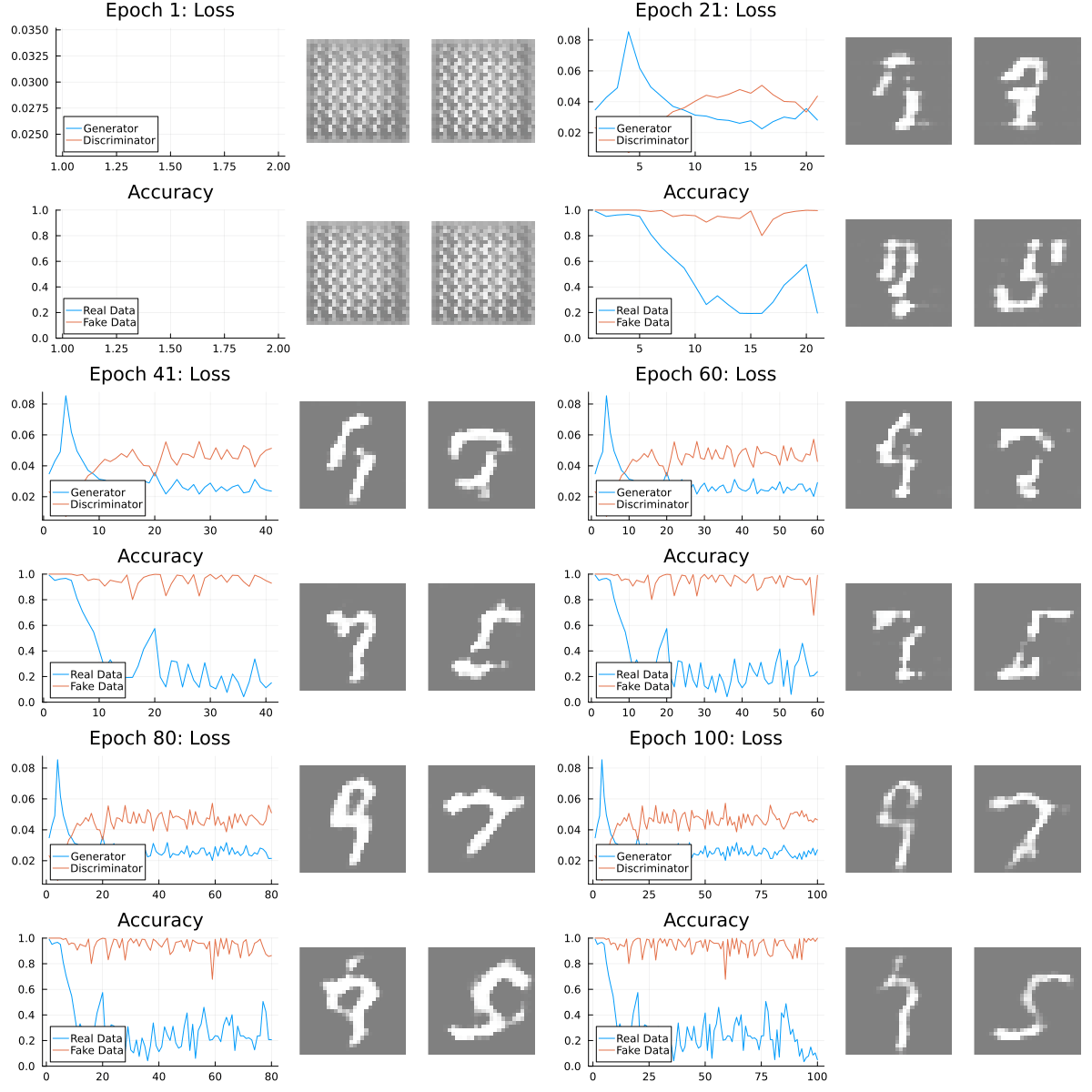
• GANs should be monitored.

• Leverage your visual system: loss, discriminator accuracy, and generated data.

• Generator and discriminator loss should be separated.

• Real and fake accuracy should be separated.

Regularisation

• Mode collapse is often related to Lipschitz continuity being violated in the discriminator: gradient penalty mechanism.

• Weight normalisation is often performed through Spectral Normalisation: \[ L += \sqrt{\Vert W \Vert_1 \Vert W \Vert_\infty} \]

Regularisation Tricks

• Discriminator is trained with multiple updates for each generator update.

• Wasserstein loss (Earth Movers Distance) redefines the game to arbitrary maximimisation - not classification.

• Usual regularisation on individual networks: dropout, early stopping etc.

Data Augmentation

• A useful feature of GANs is data augmentation: supplementing data when there is none.

• We simply generate data by sampling in the latent space and passing it through the generator.

• This is only useful when we are certain the GAN has converged correctly -serious error potential.

• Any mismatch between reality and generator will carry to downstream analysis.

Problem: How to control variance?

• A problem in experimental sciences: day-to-day variance, and experimenter-experimenter variance.

• Same underlying biology (or other natural phenomena).

• We would like to remove the bias introduce by different experiments.

Batch Equalisation

• A modern approach is to use GANs as a style transfer for data.

• The batch data is passed through a generator to look like “real” data which is trained concurrently with a generator.

• This removes the inter-batch variance and cleans up the dataset.

Summary

• A GAN is a two-player game between a generator model and a discriminator model.

• The discriminator classifies real/fake data and the generator plays to trick it.

• The game is globally minimised when the generator matches the data-generating distribution.

• The generator can be used to analyse a distribution, augment/generate data, and normalise datasets.

References

Generative Adversarial Nets, Goodfellow et. al. (2014)

Wasserstein generative adversarial networks, Arkovsky et. al. (2017)

Batch equalization with a generative adversarial network, Qian et. al. (2020)